Visualizing real-world networks often presents two intertwined challenges: (1) the visualization must reveal the distinctive structural and temporal characteristics of complex data, and (2) it must do so with a sufficient degree of clarity to make it meaningful. Here are some steps to optimize network layout in CiteSpace for users to focus on extracting valuable insights from the evolving patterns embedded in dynamic networks.

Created: 7/25/2025

Last Modified: 7/26/2025

Configuration

Project Properties

Link Retaining Factor (LRF) controls the sparsity of a network to be visualized. It retains the most important links and discards the rest of links. When LRF approaches to 1.0, the resultant network has the same number of links as a minimum spanning tree. When it is set to -1.0, all links are included. A good starting point is 1.2, the resultant network is more like a Pathfinder network.

L/N defines the maximum number of links per node. In our example, we set L/N to 35, which means we ask CiteSpace to retain up to 35 the strongest links between a given node and other nodes in the network. If you want to turn off this parameter, set it to -1.

Look Back Years (LBY) filters out long-range links over a time span from the present time slice back in time. In our example, we set LBY to 10, which means we ask CiteSpace to filter out citations to publications more than 10 years old. Again, if you want to turn off this filter, set it to -1.

Node Types

Let's make a hybrid network that consists of noun phrases extracted from titles and abstracts and cited references. The option of keywords is only available in the Web of Science records from 1990. Noun phrases would be a convenient substitute if you are interested in keyword-like patterns prior to 1990 in your dataset.

Selection Criteria

The recommended choice is g-index. You can scale the selected set up or down by the scale factor k. In this example, k is 100.

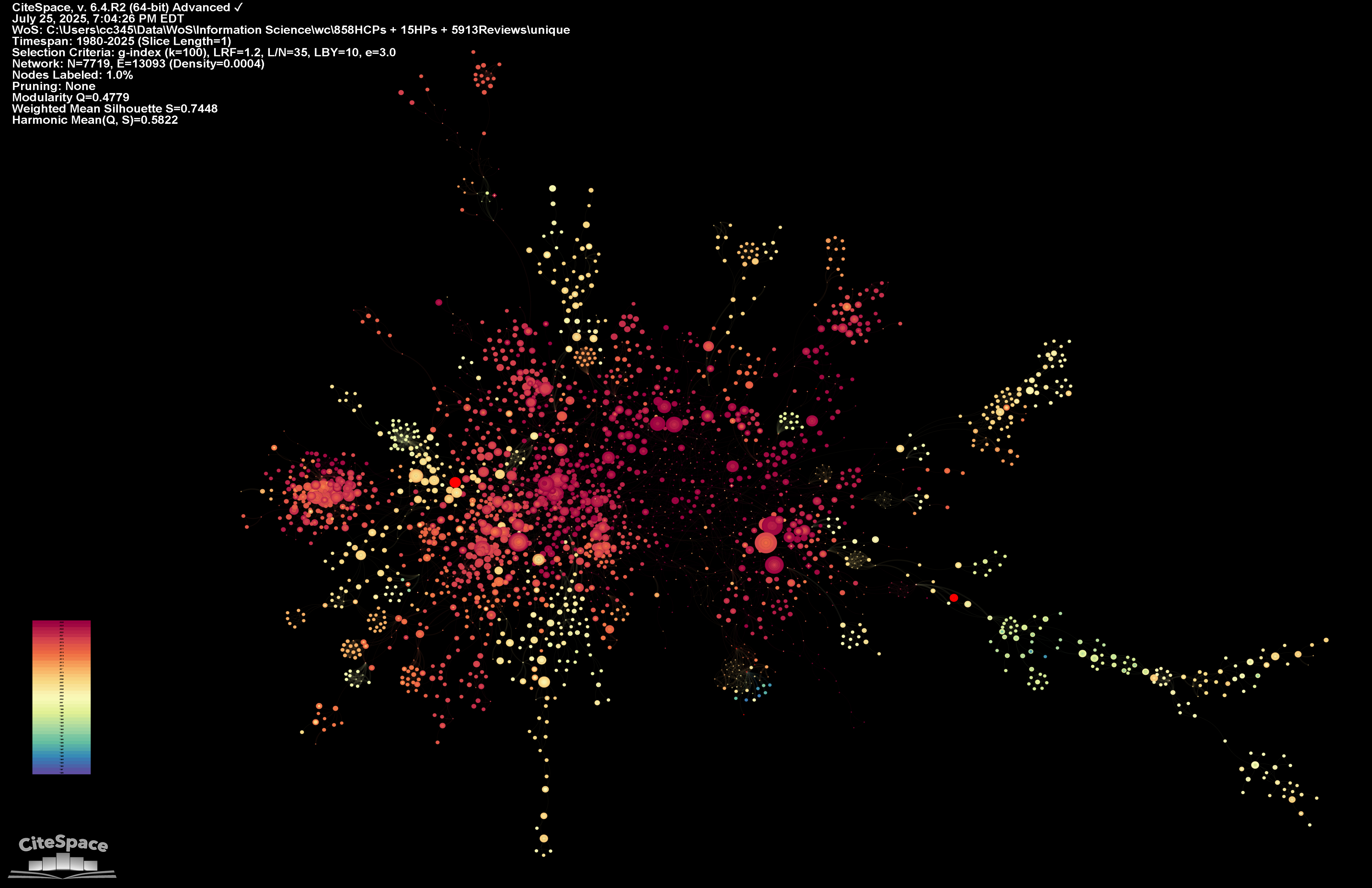
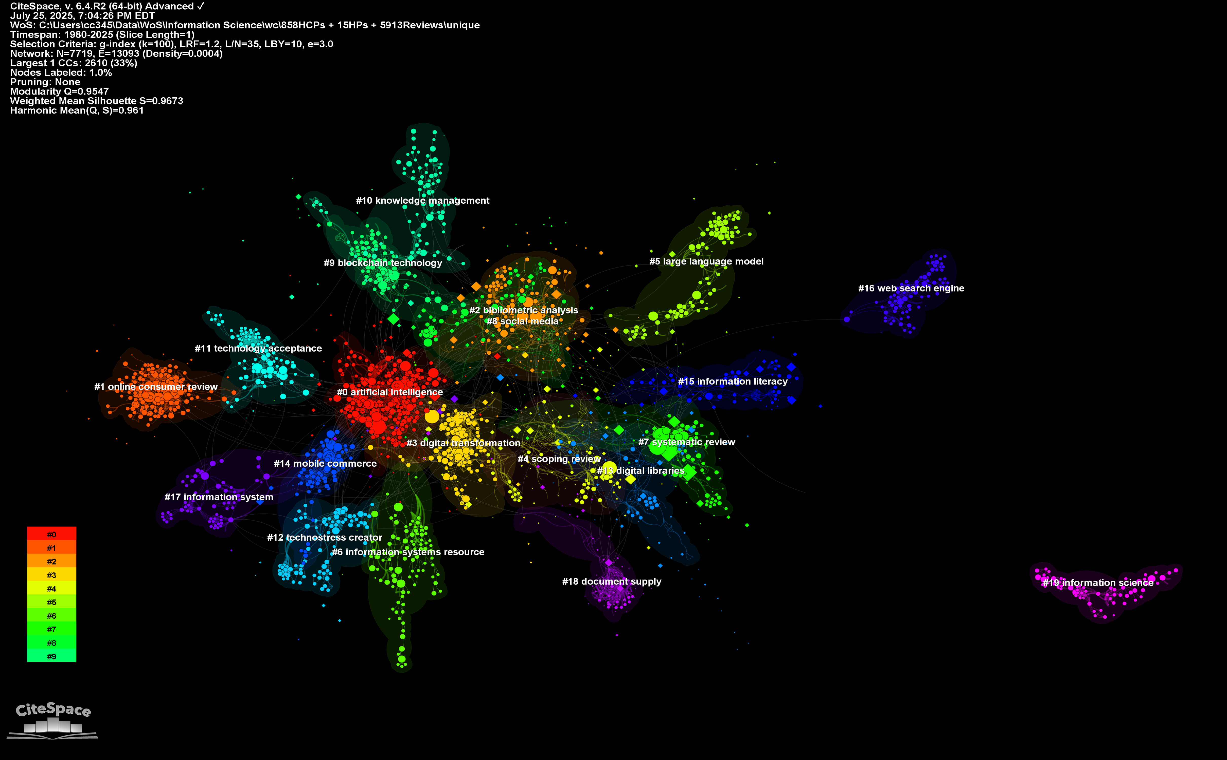
Initial Layout

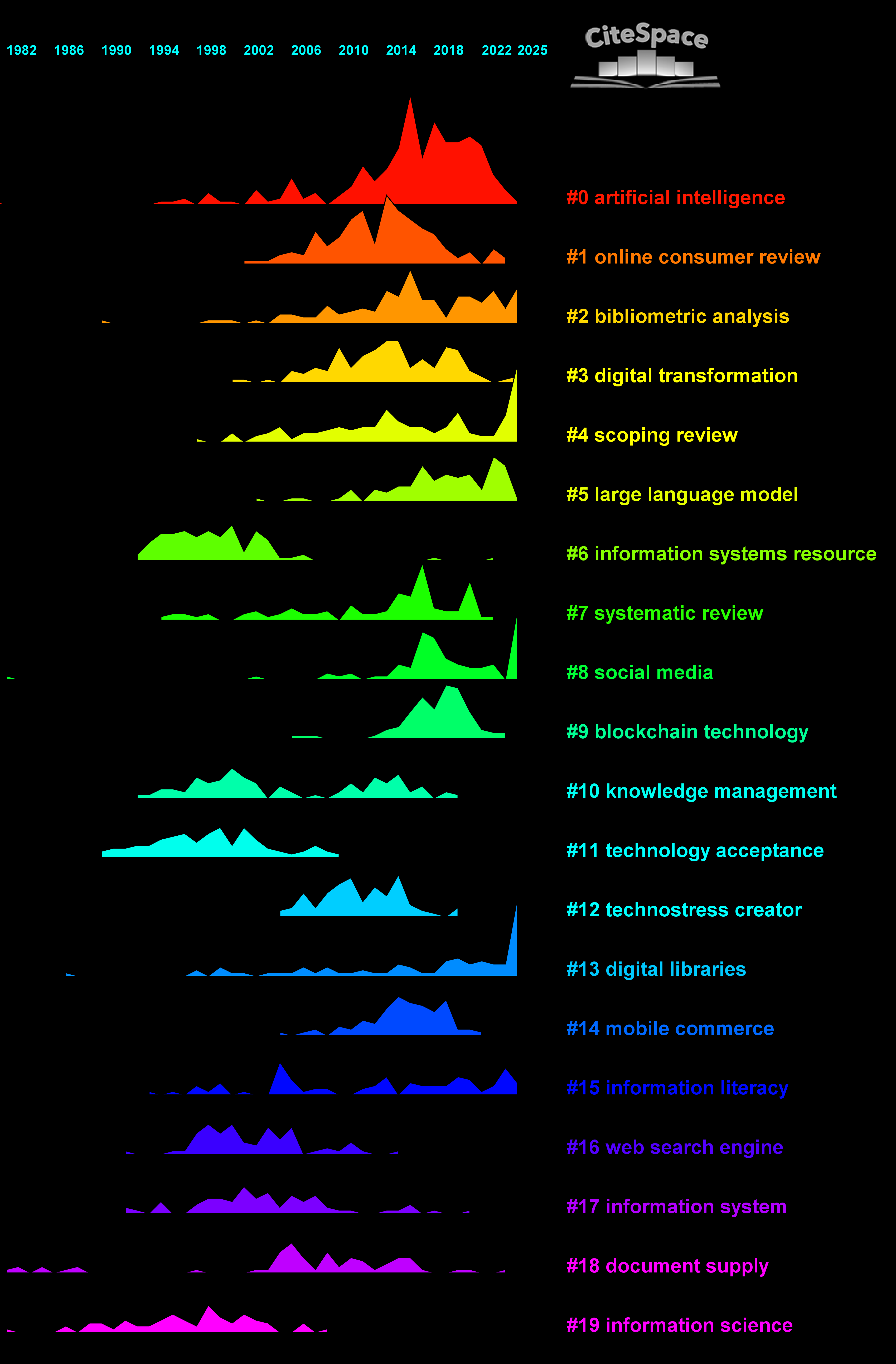
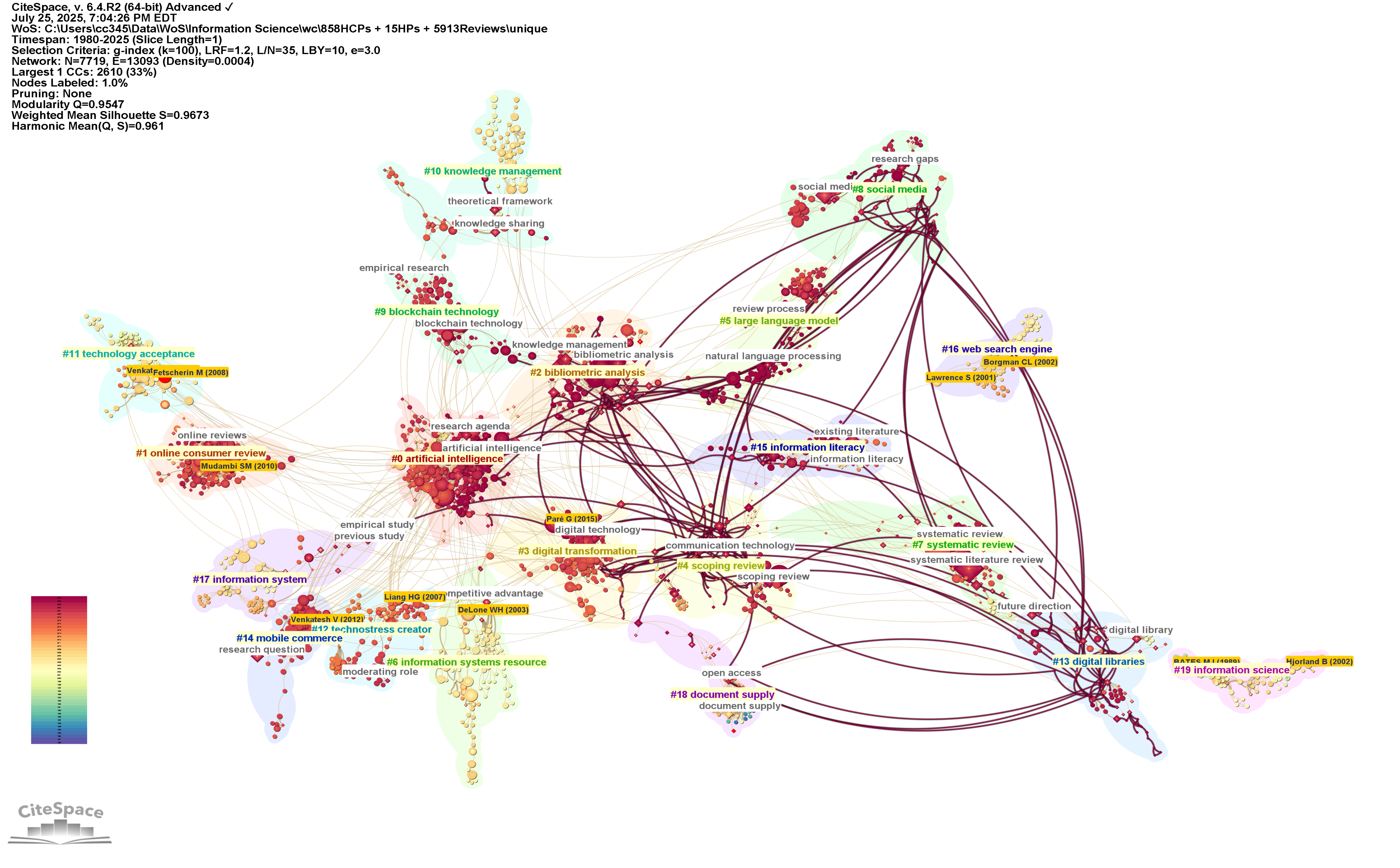
Here is the initial layout of the network. It looks like a tree as we expected. The colors represent the time of citations to an article. This is a tree-ring view, where the size of a node depicts the citations it received. The larger the circle, the more prominent the underlying article is.

Clustering

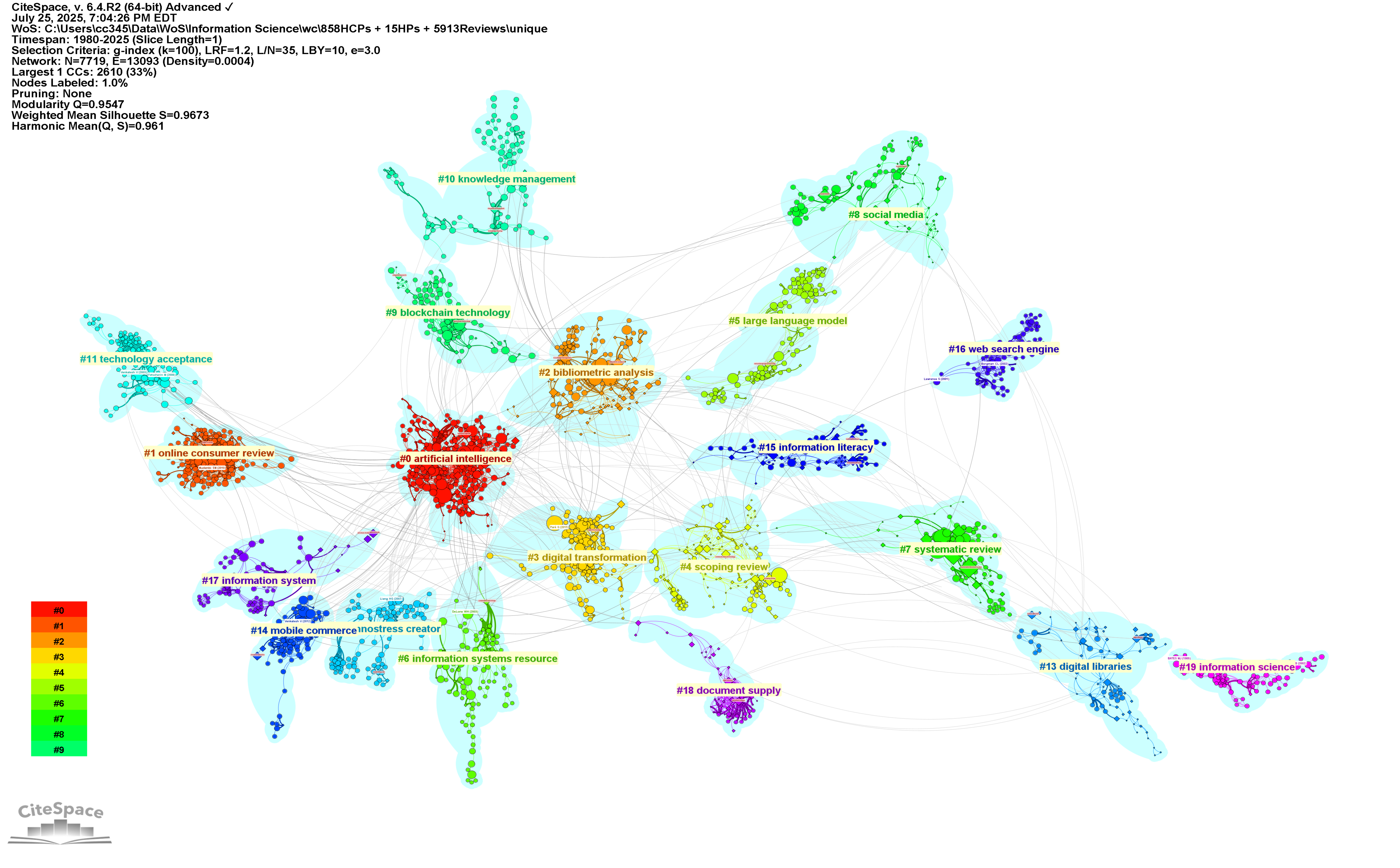
More insights can be revealed by dividing the network to clusters. You have two options here: do you want to preserve the current layout? For the demonstration sake, let's preserve the layout first and then we will show what layout optimizations are possible.

To generate clusters without altering the current layout, use Find Clusters under the Clusters menu:

Nodes in the same cluster have the same color. The largest cluster is in red. The coloring is based on a rainbow colormap. Yes, we know how a rainbow colormap could be harmful, but not in this case.

Optimize Layout

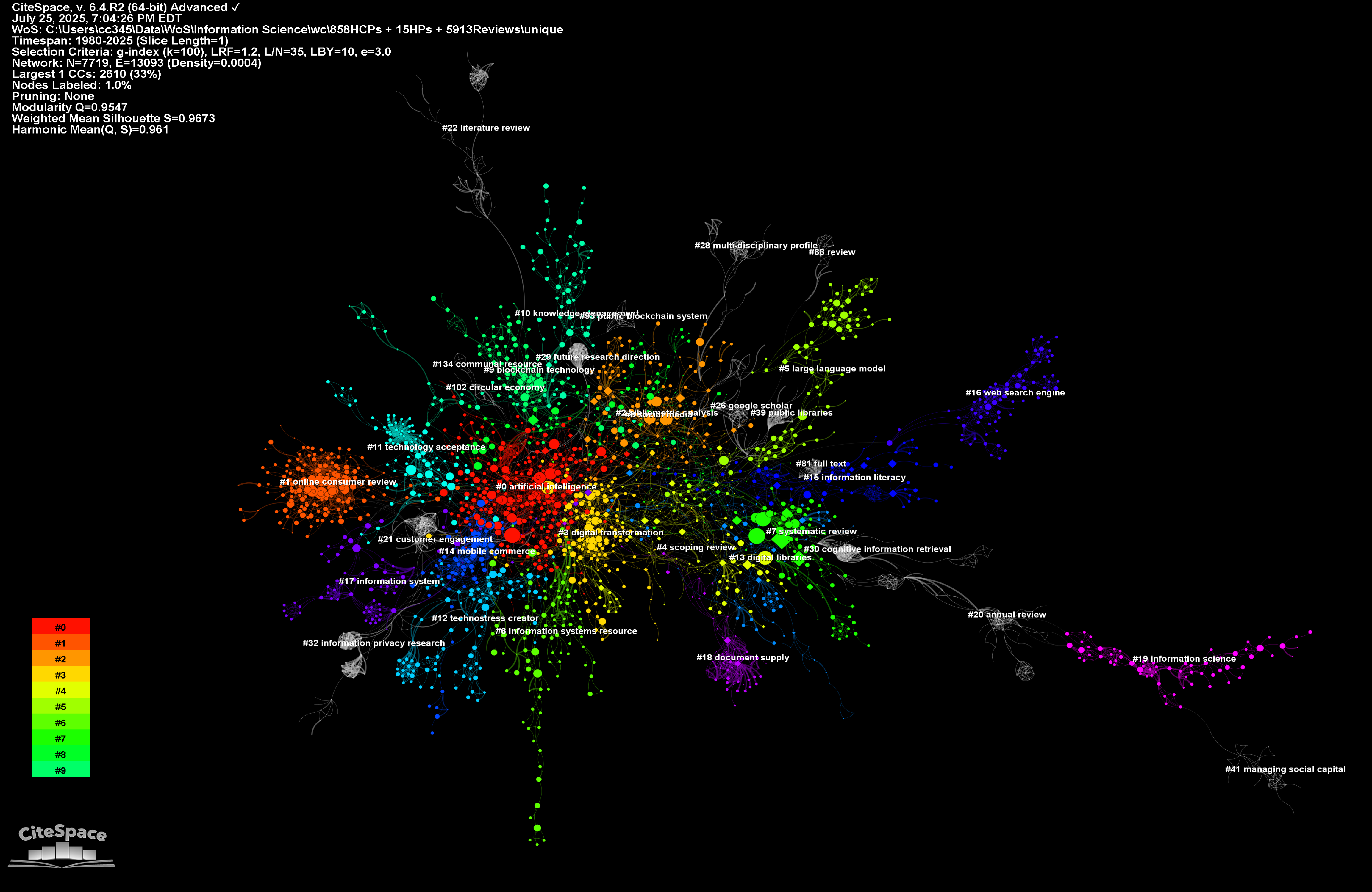
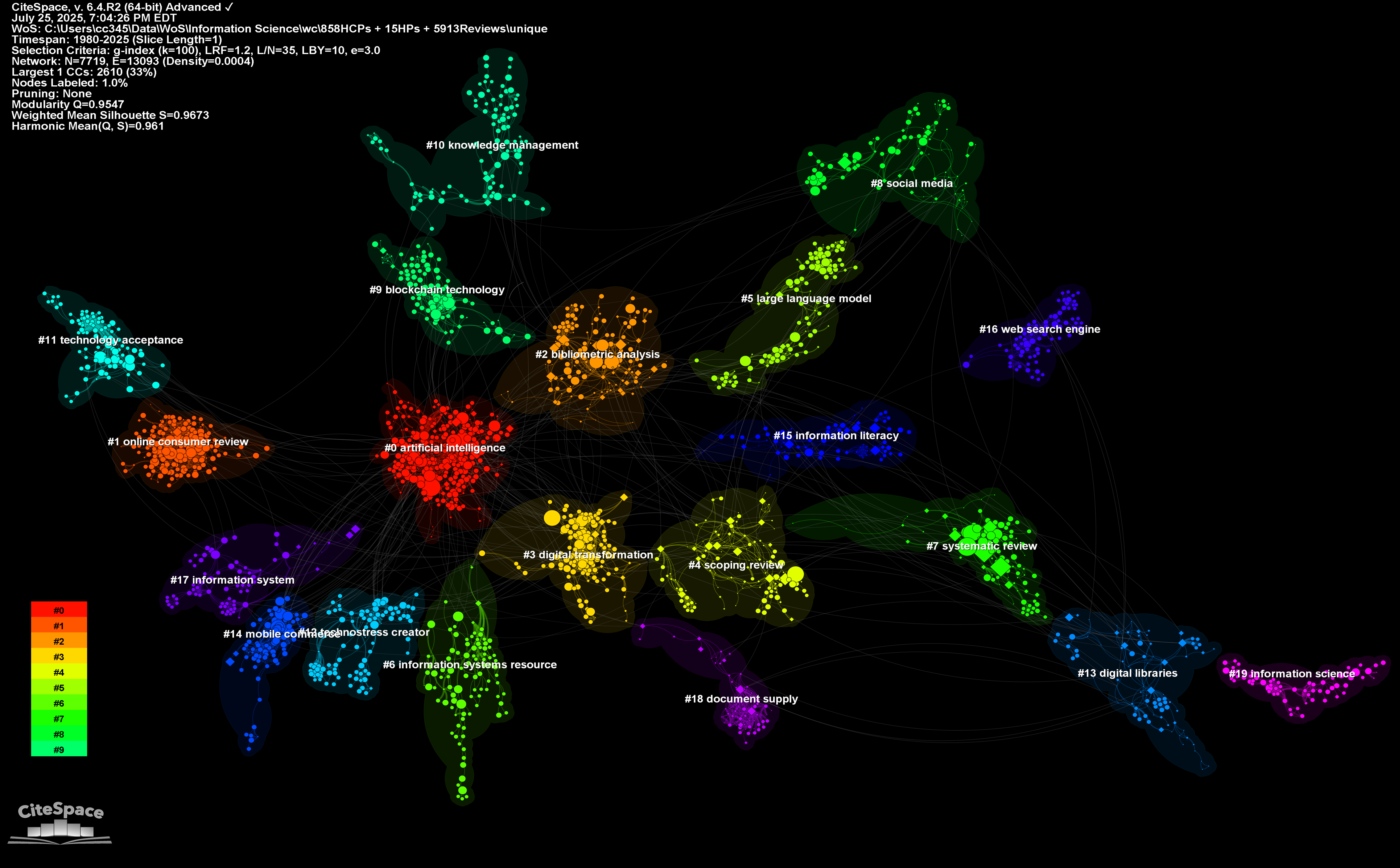
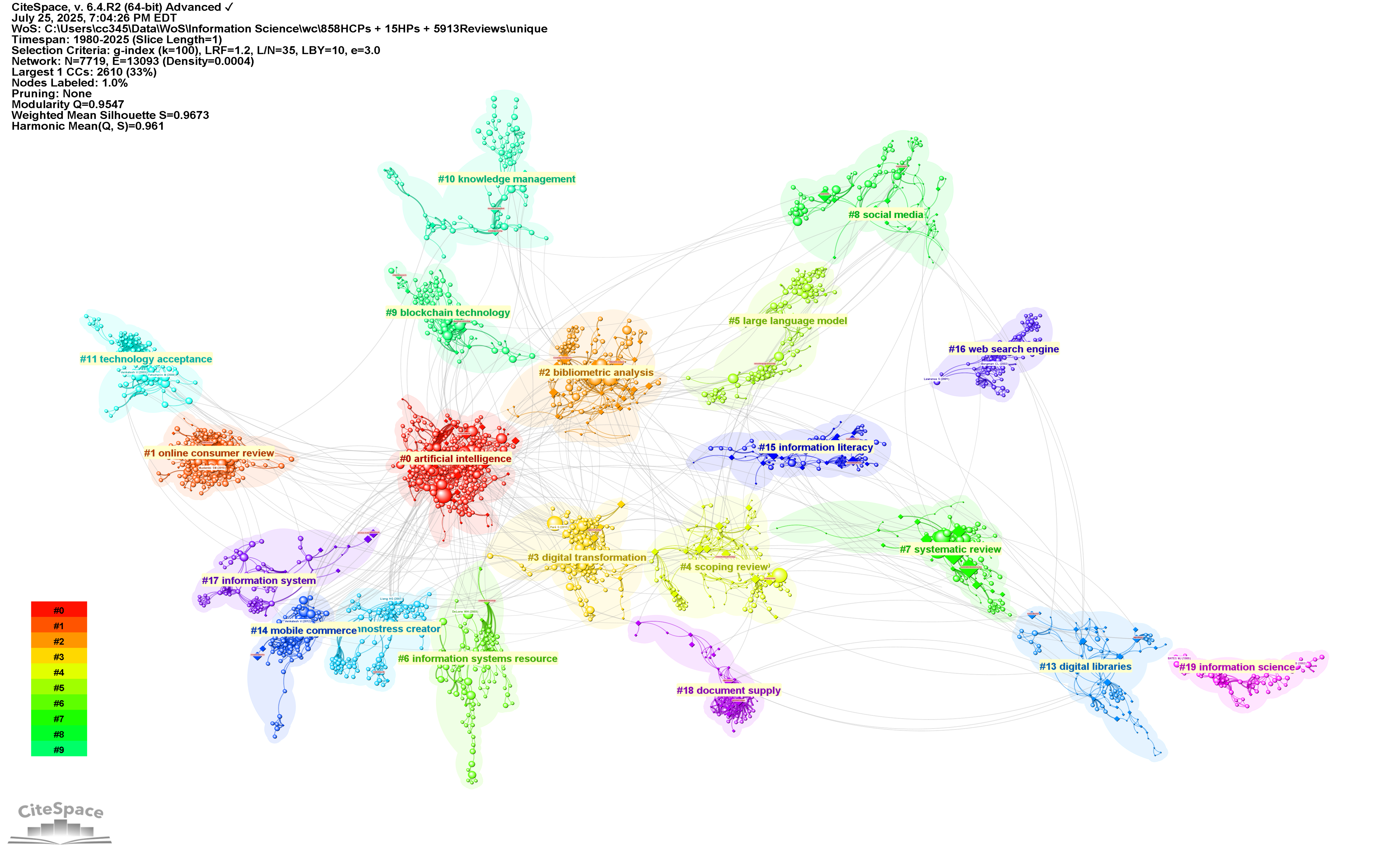
The All in One function, the middle one shown in the figure below, does a few things together, including generating cluster labels and optimizing the layout.

The optimized layout separates overlapping clusters while preserving the layout of each individual cluster. In other words, the shape of a cluster remains the same.

Sometimes The All in One function may not fully separate overlapping clusters. If you are a perfectionist, you may increase the separation further by using the Optimize Layout function under the Clusters menu and you can repeat the function until they are fully separated.

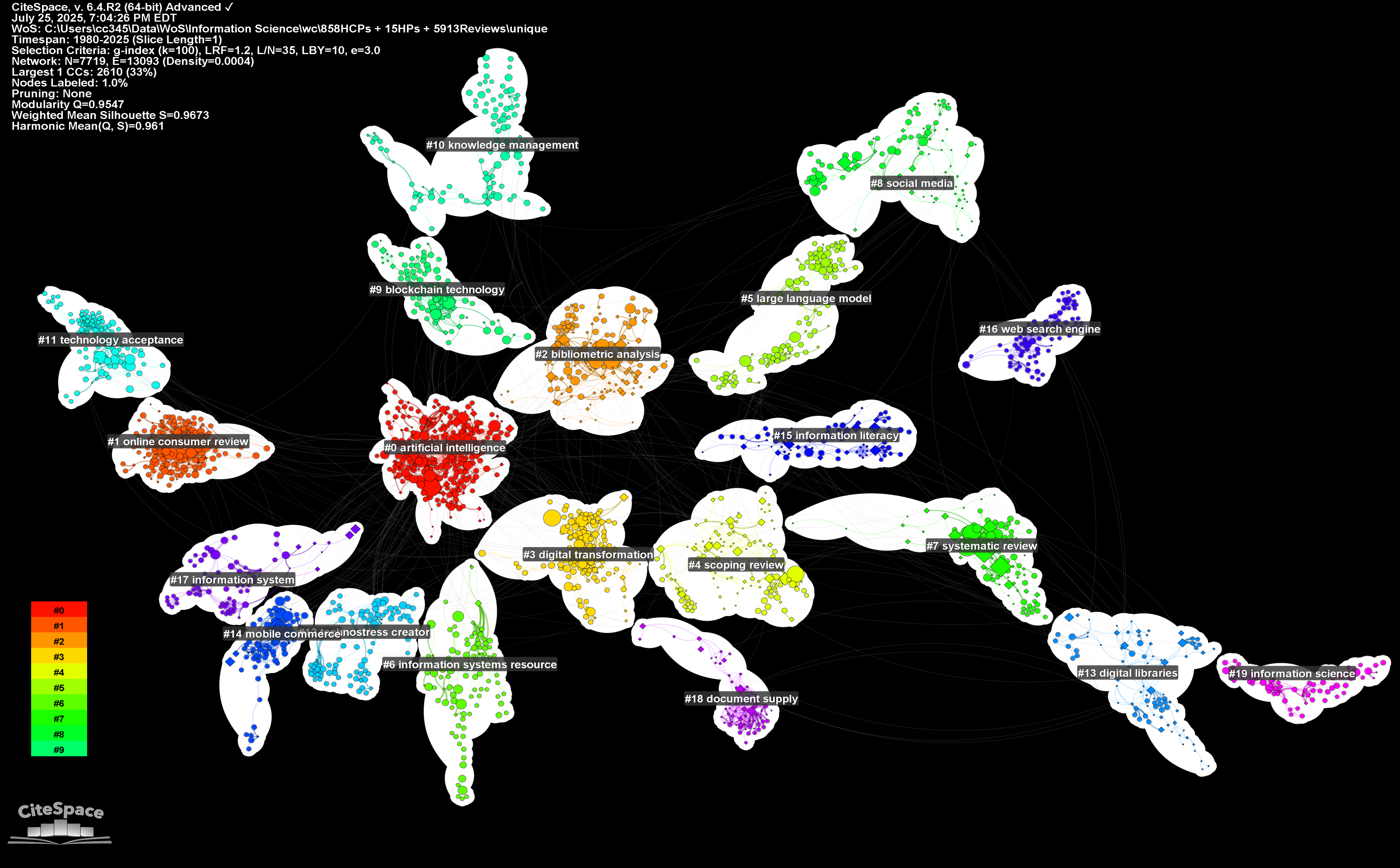
The Background Color of a Cluster

To make it easier to see the groupings of a cluster, CiteSpace outlines individual clusters with colored areas that track their shapes. You can set a universal color for all the clusters such as the white color in the example below.

You may select a fill color as you like. For example, you can change the overall background color to white and select a different color accordingly.

Alternatively, you can keep the default setting, which matches the cluster background color to each cluster as shown in the example below.

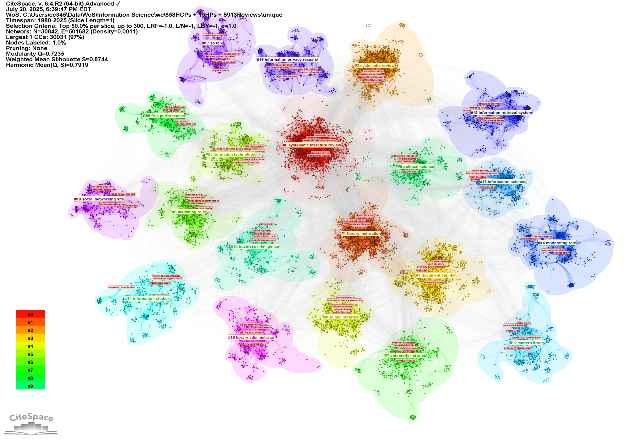
A Vertically Repeatable Method

Here is another hybrid network. Its largest connected component alone has over 30,000 nodes. Layout optimizations that preserve the internal structure of clusters are particularly helpful as several clusters are tightly coupled with a strong inter-cluster linkage. This example illustrates how the layout optimization strategy can help us to break down an otherwise dense hairballs to reveal its complex structure in a meaningful way. Furthermore, CiteSpace allows you to examine an individual cluster of your interest by applying the same procedure to the cluster as if it is the entire network of its own. One can repeat the same procedure again and again until clusters with a sufficient level of homogeneity are reached.

Manual Adjustments

CiteSpace allows you to make manual adjustments to the layout. Select the Cluster Move Mode under the Clusters menu. It allows you to move one cluster at a time by dragging any of its member node. You may use Cluster Dependencies as your guide. In general, you should only move a cluster to reduce the length of a cluster dependency link. In principle, keep such adjustments to the minimum for a better reproducibility and simplicity. Afterall, just because we can take a step does not necessarily mean it is the best move.

Display Multiple Layers of Information

Once an optimized layout is in place, we can interact with the visualized network by cross-referencing multiple layers of information at a finer granularity level. In the hybrid network, for example, the prominent terms and cited references in each cluster provide more specific information. The year-by-year tree rings encode the history of individual publications.

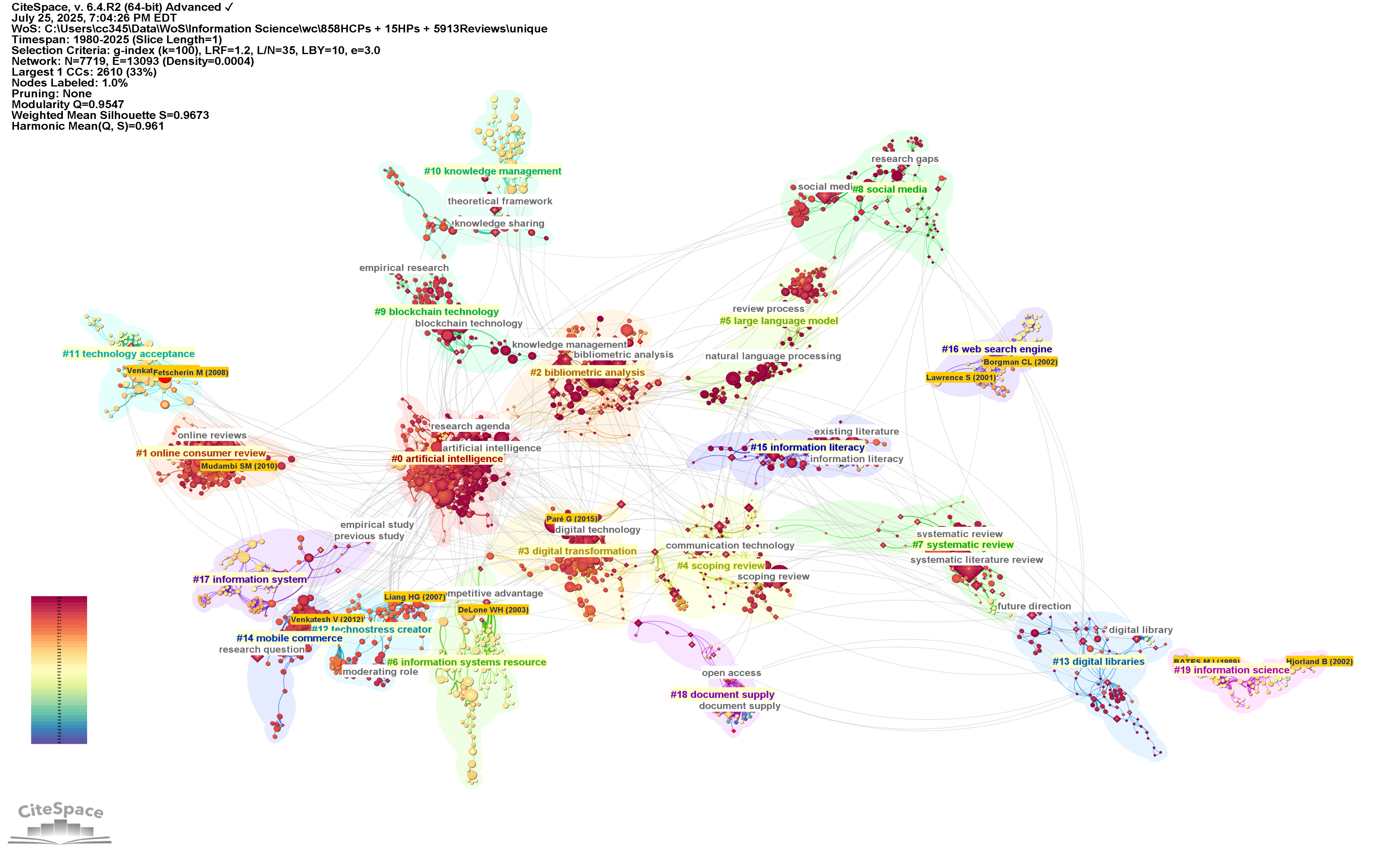
The Link Walkthrough function steps through the snapshots over time so that we can see how connections between various clusters evolve at a particular point of time. Each click moves one period of the time slicing length you choose. If you choose monthly time slicing instead of the default yearly slicing, then the function steps through the network monthly, which can be helpful when you are dealing with a rapidly advancing domain of research, for example, in the cases of COVID-19 and ChatGPT. You can move forward and backward. The following is a snapshot of July 2025.

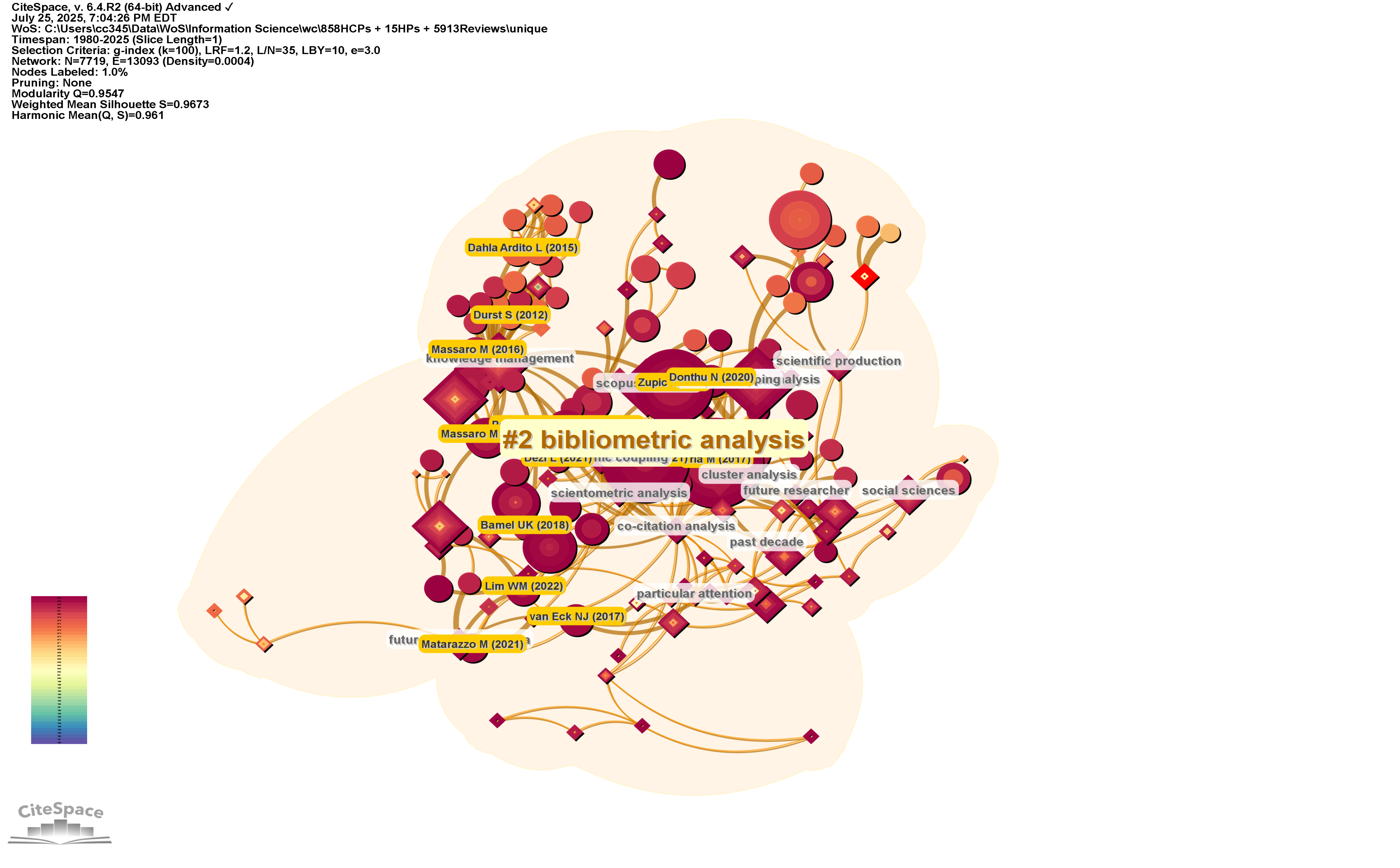
We can zoom in to a particular cluster such as Cluster # bibliometric analysis to explore the cluster at the level of its membership.

There are deeper theoretical foundations behind these analytic tasks, what we should look for, and what they mean. I will cover them in another blog.

Cross-Reference with Other Views

The cluster view we have demonstrated above is a valuable source of insights. Nevertheless, CiteSpace also offers other views such as timeline view, circular view, heat map view, and landscape view. Considering these views side by side can help us uncover more insightful patterns and signals and develop a better understanding of the underlying field of study.